
Machine Learning - Supervised Learning Algorithms Comparison
Introduction
Supervised learning is a subset of machine learning that can also be broadly defined as function approximation. Functions are approximated using induction on labeled training data of input-output pairs of datasets. Several different algorithms and methods of supervised learning exist, and hyperparameters of each algorithm can govern their specific behaviour and performance. The purpose of this project is to explore, study, analyze and gain a deeper understanding of supervised learning methods through experimentation and analysis.
Methods
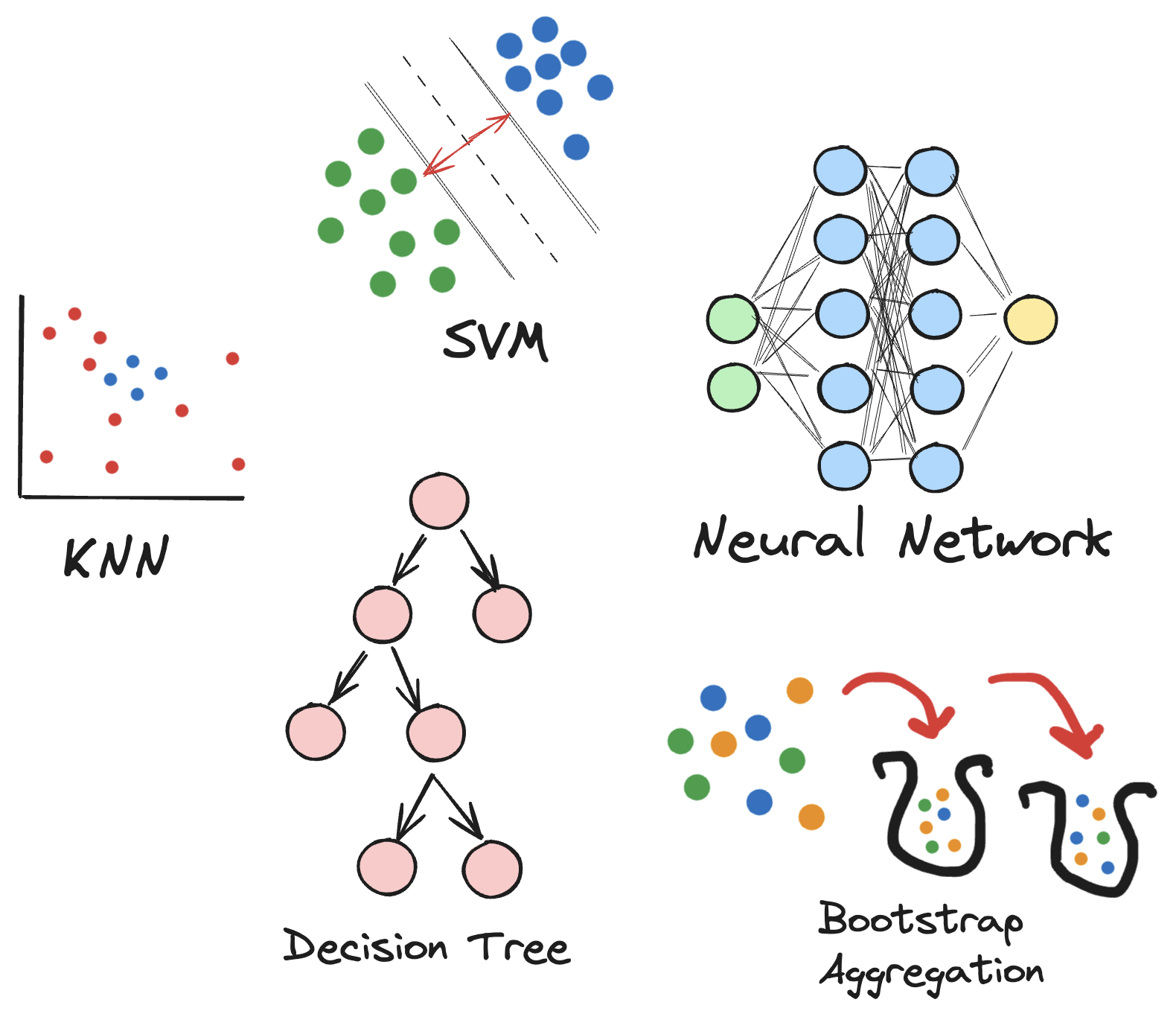
In this project, five different learning algorithms were studied: Decision Trees, Neural Networks, Boosting (Bootstrap Aggregation), Support Vector Machines, and K-Nearest Neighbours. Two labeled classification datasets were selected for which each of the learners were trained and assessed on. Each dataset was split into a training set (70%) and a test set (30%). Learning curves were generated for each dataset-algorithm pair, whereby k-folds operations were performed (k=5) on the training set for cross-validation scoring. For each algorithm, two hyperparameters were selected for isolated tuning in order to study its effect on various aspects of the algorithm, as well as to better dissect the algorithm itself with respect to how the hyperparameter impacts its performance and behavior. The primary metrics used to compare each algorithm included training time, learning rates, and classification scoring. Additionally, confusion matrices of the overall performance were provided for some outputs. These metrics were used to analyze the different characteristics of the various algorithms which are discussed throughout the report.
For each of the algorithm-dataset pairs, hyperparameters were selected by running a grid-search algorithm. From there, manual tuning was conducted. The hyperparameter values are presented in the results section for each run. Implementation of each algorithm was conducted using Python and Scikit-Learn libraries. All runs were completed with a constant seed in order to control for randomness.
Datasets
Two Labeled Classification Datasets
Two labeled classification datasets were selected for testing and experimentation. These datasets differ in a multitude of ways, as discussed below. The intention behind selecting datasets that differ in several ways is driven by the goal of eliciting differences in behavior and performance across the selected algorithms in order to better highlight and understand algorithmic differences.
Handwritten Digits Data Set
The first dataset selected is a handwritten digits dataset 1. Each image is 8x8 pixels, where each pixel is considered a feature. There are thus 64 features, and the value of each represents the intensity of the pixel as a real number between 0.0 and 1.0 (0 being black, and 1 being white). The classification target consists of the set [0, 1, 2, 3, 4, 5, 6, 7, 8, 9]. The dataset is balanced, in that the number of samples for each class is approximately the same. The total number of samples in this dataset is 3823.
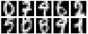
Figure 1: Visualization of different digits samples
This dataset was considered interesting from a machine learning perspective for a number of reasons:
- Human readers are easily capable of visually classifying most of the samples themselves without being aware of exactly how their brain does so.
- Images tend to contain a large degree of noise.
- Correct classification often depends on higher-order factors such as shape/structure, not just feature values (individual pixel intensities).
- It has a relatively large number of features (64), 10 possible outputs, and a relatively small number of samples (3823).
Accuracy was selected as the performance metric for the training dataset because the dataset is balanced, and because it’s an intuitive measure of success.
Adult Income Prediction Dataset
This dataset 2 consists of 16 features where each row represents a person. Features include discrete traits like ethnicity, country of origin, and education level, as well as continuous features such as income and age. The class being predicted is whether an individual has a salary of greater or less than $50,000 USD each year. This dataset was selected to contrast the digits dataset, as it differs in several ways. For instance, the target class output is binary, the dataset is unbalanced (25% > 50k, 75% <= 50k), and the number of features is comparatively small (16), while the number of samples is comparatively large (approx. 30,000).
Pre-processing of this dataset involved removing rows that had null entries, and one-hot encoding of all discrete features. Additionally, all continuous features were normalized to a real number between 0 and 1.
F1 Score was selected as the performance metric for all training on this dataset since it is unbalanced. If accuracy were to be selected, a learner could produce a 75% accuracy score by always guessing <= 50k. The F1 Score is therefore a more appropriate performance metric as it combines recall and precision into a single metric. It should be noted, however, that in overall performance comparison, both F1 Score and Accuracy of the end results were used.
Decision Trees
Dataset 1: Digits
| Splitting Criterion | Gini |
|---|---|
| Max Depth | 20 |
| Max Features | None |
| Max Leaf Nodes | None |
| Min Samples Per Leaf | 1 |
| Min Samples Per Split | 2 |
Table 1: Hyperparameter Values - Decision Tree - Digits Dataset
The parameters selected by this search were experientially (and through grid search) determined. However, these values allowed the decision tree to grow infinitely until it matches the training data exactly, thus overfitting. Despite the propensity toward higher bias, the maximum cross-validation scores were found values that allowed overfitting.
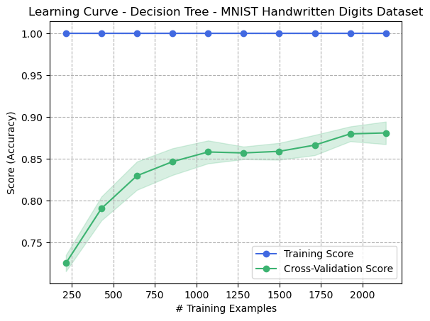
Figure 1: Learning Curve - Decision Tree - Digits Dataset
The learning curve demonstrates that more samples corresponded with greater cross-validation performance. However, the model was still biased toward the training set in all cases since the learner performed with perfect accuracy on the training set. This indicates that the model is overfitting the dataset.
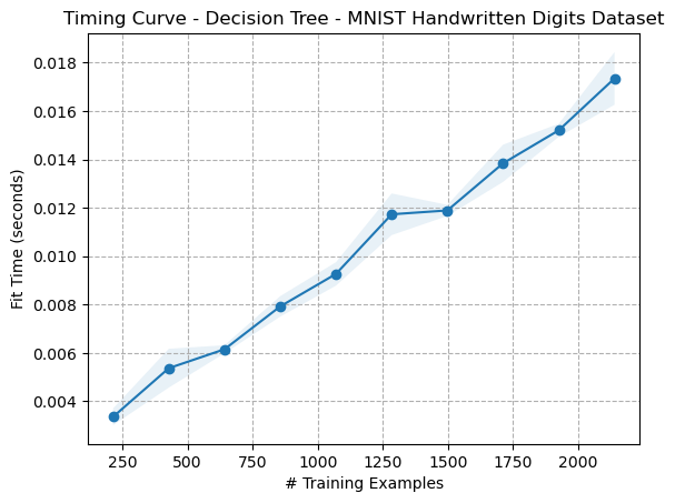
Figure 2: Timing Curve - Decision Tree - Digits Dataset
The timing curves for both datasets appear that the fit time increases linearly, or (O(n)) or perhaps logarithmically. Decision Trees’ average fit time complexity is (O(n \log(n))), so the results appear to match theory.
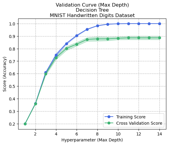
Figure 3: Validation Curve - Max Depth - Decision Tree - Digits Dataset
Figure 3 shows the effects of tuning the maximum depth of the decision tree. This graph demonstrates that increasing the maximum depth of the tree tends to cause overfitting to occur, since a tree can be created which fits the training data perfectly. This graph depicts an example of overfitting and the bias-variance trade-off, whereby the model continuously proves to be more accurate overall at the expense of increasing the overall bias toward the training data.
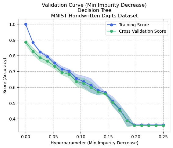
Figure 4: Validation Curve - Min Impurity Decrease - Decision Tree - Digits Dataset
Figure 4 shows the effects of tuning the minimum impurity decrease. This hyperparameter controls how much information gain must occur in order to consider the splitting of a node. In this case, the Gini index is used. Minimizing this parameter (0.0) allows any amount of information gain to result in a node splitting, and therefore would allow the generation of a tree that perfectly matches the training data. The figure confirms this hypothesis, as the training accuracy of the model is 100% when this index is set to 0.0, and gradually decreases as the value increases. This corresponds to smaller trees being generated, which are also considered more generalized (less overfit) models since the variance decreases along with the bias. Overfitting implies that the model is overly complex and has learned the noise and random fluctuations in the training data rather than the underlying patterns. It is notable that in both cases of hyperparameter tuning, any reduction in the complexity of the Decision Tree (to generalize it and reduce overfitting) tended to also cause its cross-validation score to drop. This is because by reducing the size of the tree, or by pruning, it is likely removing some of the information that the tree has learned. While some of those pruned branches may have captured noise that led to overfitting, they may have also contained useful patterns as well which is why the lost complexity also performed worse on unseen data.
Dataset 2: Adult Income Prediction
| Splitting Criterion | Gini |
|---|---|
| Max Depth | 15 |
| Max Features | None |
| Max Leaf Nodes | 40 |
| Min Samples Per Leaf | 1 |
| Min Samples Per Split | 2 |
Table 2: Hyperparameter Values - Decision Tree - Adult Dataset
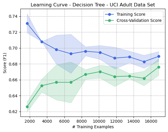
Figure 5: Learning Curve - Decision Tree - Adult Dataset
Figure 5 shows an interesting trend in that increasing the number of training samples reduces the variance between the training score and the cross-validation score. In this example, as the bias toward the training data decreases, the variance decreases since the cross-validation score improves. The fact that the training data was never capable of reaching an F1 score of 1.0 suggests that a Decision Tree could not be generated which perfectly matched all training data, which might indicate noise in the dataset or perhaps weak correlations. This would intuitively seem correct as the features alone (age, ethnicity, country of origin, etc) are unlikely to be perfect predictors of income, and thus no set of concrete rules can be learned to predict with perfect accuracy. Generalization in Decision Trees is typically achieved by limiting the size of the tree in some way, which can be seen in the hyperparameters having been set (Max Depth of 15, Max Leaf Nodes of 40) which prevents it from biasing too heavily on training data.
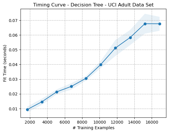
Figure 6: Timing Curve - Decision Tree - Adult Dataset
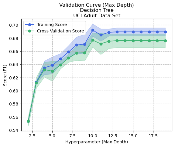
Figure 7: Validation Curve - Max Depth - Decision Tree - Adult Dataset
Varying the maximum depth of the tree showed interesting behavior. Whereas the cross-validation score benefited with ever-increasing max-depth in the Digits dataset, this dataset appeared to perform better overall with a maximum depth having been limited at 10. If a decision tree model with a smaller maximum depth performs better on a dataset compared to one with unlimited depth, it might mean that the dataset contains noisy data or has a high degree of variance.
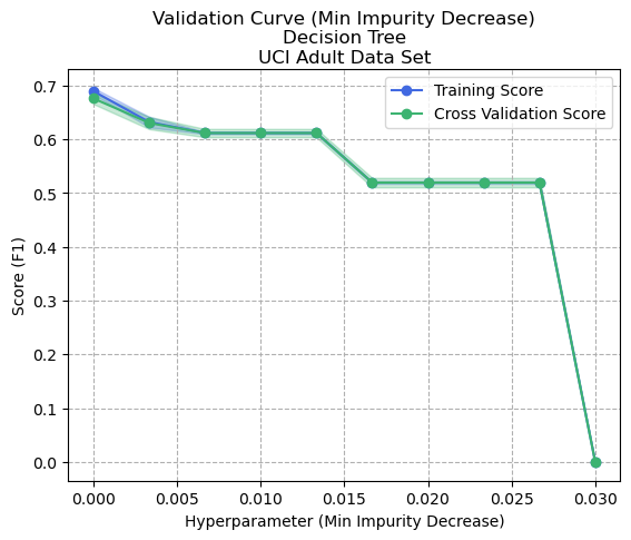
Figure 8: Validation Curve - Min Impurity Decrease - Decision Tree - Adult Dataset
Adjusting the minimum impurity decrease as per Figure 8 showed a decrease in bias, since the performance metric on training data and on cross-validation data matched when it was set to 0.003. However, the performance overall suffered so it was considered more optimal to keep the value at 0, thus accepting some overfitting.
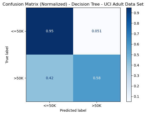
Figure 9: Confusion Matrix - Decision Tree - Adult Dataset
The normalized confusion matrix was included to demonstrate that while the model tended to successfully predict the more common class (<= 50k) most of the time (95%), it could only correctly predict the other class (>50k) 58% of the time. This could indicate that a considerable amount of noise exists in features for this class which the single Decision Trees could not adequately capture. Noise in a dataset could prevent splitting on specific values for features from producing information gain (Gini or reduction in entropy), which could explain its difficulty in successfully predicting this class.
Boosting
Dataset 1: Digits
| Weak Learner | Decision Tree (Max Depth = 2) |
|---|---|
| Number of Weak Learners | 500 |
| Learning Rate | 0.5 |
Table 1: Hyperparameter Values - Boosting - Digits and Adult Dataset
Boosting was completed with the parameters specified in Table 1 for both datasets. The weak learner selected was a Decision Tree with a maximum depth of 2. Boosting algorithms can be viewed as a gradient descent problem3, and they are interesting because they tend to not overfit as long as the weak learners cannot independently overfit4. By training the trees on the residuals or errors made by previous trees, boosting algorithms focus the attention of each new tree on the difficult examples that the previous trees struggled with.
Another factor that helps to prevent overfitting in boosting algorithms is the use of regularization. AdaBoost was used in this case, which includes a regularization term in the loss function that is optimized during training. This term penalizes complex models and helps to prevent overfitting.
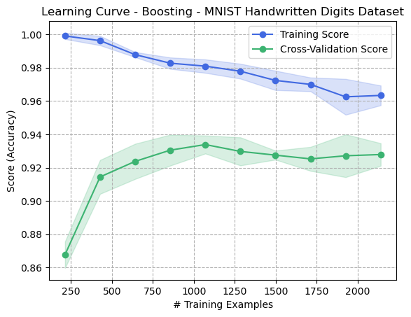 Figure 1: Learning Curve - Boosting - Digits Dataset
Figure 1 shows the learning curve for the Digits dataset and demonstrates the robustness against overfitting that the Boosting algorithm has. As the number of training examples increases, the bias decreases (avoids overfitting), but the validation score does not decrease. This can be contrasted to the Decision Tree learning curve (Figure 2) where the Decision Tree was allowed to grow infinitely to match (overfit) the training data exactly. In the case of Boosting, weak learners of depth 2 were used, none of which are capable of perfectly fitting the input training data. This helps explain why the boosting algorithm tended to not overfit.
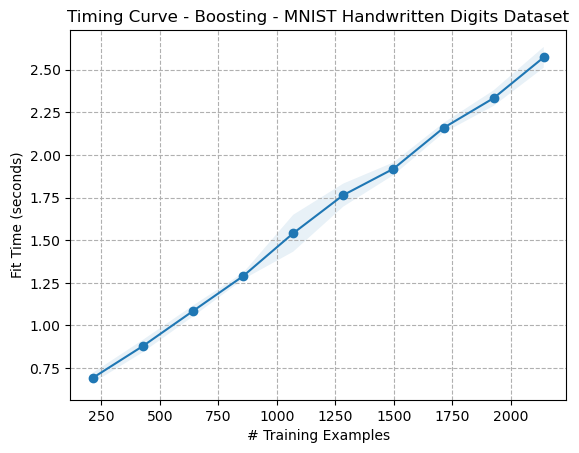 Figure 2: Timing Curve - Boosting - Digits Dataset
The timing curves for boosting (Figures 2 and 6) are interestingly of similar shape to their Decision Tree counterparts (Figures 3 and 7). However, while they appear to have the same time complexity, the boosting timing curves are noticeably an order of magnitude larger. This is likely because, while the time complexity of an individual Decision Tree is (O(mn \log(n))), where (m) is the number of features, the time complexity of Boosting with Decision Tree weak learners is (O(Tmn \log(n))), where (T) is the number of boosting rounds5. This explains why boosting algorithms’ timing curves appear to take some constant multiplier longer, as it’s likely due to the number of weak learners which remained constant.
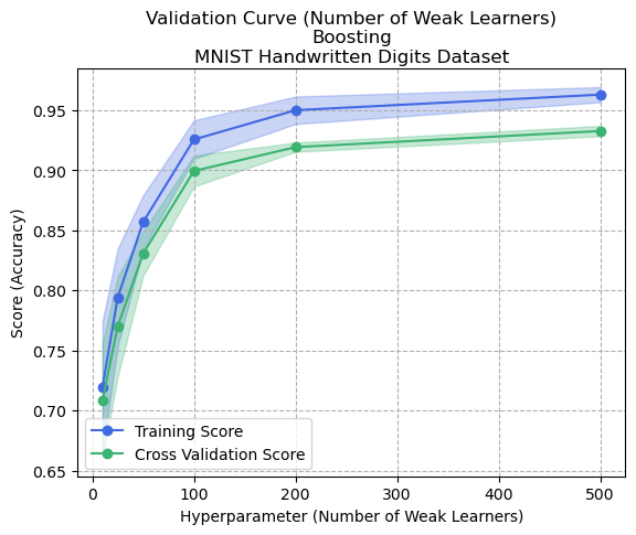 Figure 3: Validation Curve (Number of Weak Learners) - Boosting - Digits Dataset
Validation curves that tweak the number of weak learners showed interesting and differing results for both datasets (Figures 3 and 7). In the digits dataset, increasing the number of weak learners caused a plateau effect for both training and cross-validation that appeared proportionally biased for all cases. This could indicate that the dataset had less noise and was generally easier to predict with set rules. In contrast, the Adult dataset showed an interesting result where more weak learners meant greater bias and higher variance (lower cross-validation score). This could be attributed to the fact that each tree in the ensemble aims to improve the performance of the previous tree, so if the number of trees is increased, the ensemble becomes increasingly complex and can fit the training data too well, leading to overfitting. This could also mean that the model fits the training data too well, capturing not only the signal but also the noise in the data, implying that the Adult dataset contains more noise than the digits dataset.
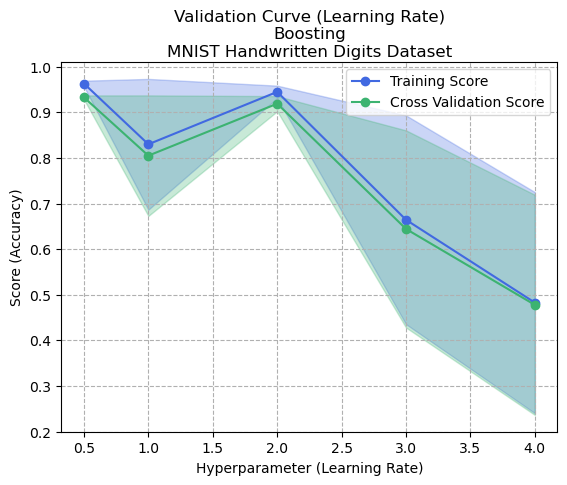 Figure 4: Learning Curve (Learning Rate) - Boosting - Digits Dataset
Figures 4 and 8 show the validation curves for controlling the learning rate of boosting. The learning rate in boosting refers to a hyperparameter that controls the contribution of each weak learner to the final ensemble, and determines the weight given to each weak learner in the final weighted average of predictions. A lower learning rate means that each weak learner contributes less to the final ensemble, and vice versa.
In boosting, the learning rate is used to trade off between the fitting of the training data and the model’s generalization ability. Low learning rates mean that the model can fit the data more closely (and possibly noise), which could result in overfitting. Too high of a learning rate could result in fast convergence and underfitting. This relationship can be seen experientially in both graphs.
Dataset 2: Adult Income Prediction
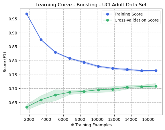 Figure 5: Learning Curve - Boosting - Adult Dataset
The Adult dataset similarly shows the benefits of Boosting to prevent overfitting, whereby the increased number of training examples tends to decrease variance and also decrease bias, since the training and validation scores appear to converge and the difference in performance decreases between the two.
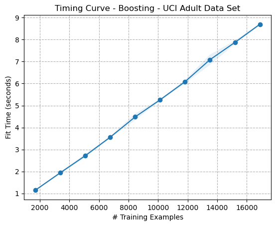 Figure 6: Timing Curve - Boosting - Adult Dataset
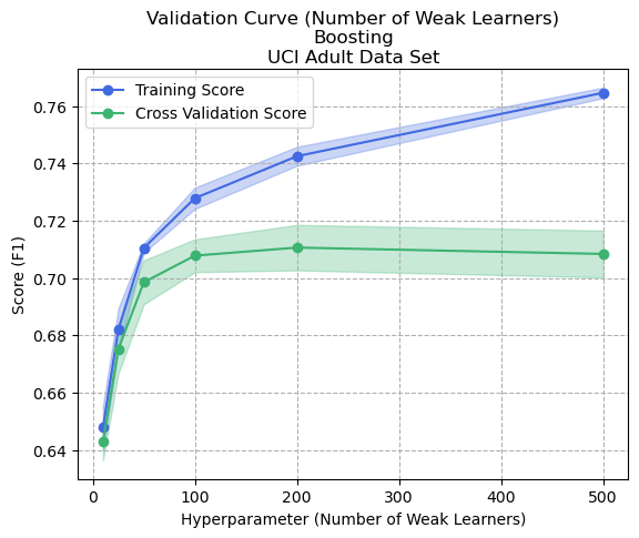 Figure 7: Validation Curve (Number of Weak Learners) - Boosting - Adult Dataset
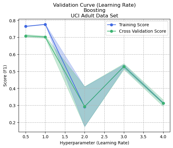 Figure 8: Validation Curve (Learning Rate) - Boosting - Adult Dataset
K-Nearest Neighbours
Here’s how the LaTeX content can be converted to Markdown with the specified image references:
Dataset 1: Digits
| Number of Neighbours (K) | 1 |
|---|---|
| Weights | Uniform |
Table: Hyperparameter Values - KNN - Digits Dataset
A KNN model was trained with the parameters specified in the table above for both datasets. K was varied during hyperparameter tuning, and ( K=1 ) was selected to provide the best performance. However, referring to the Learning Curve (Fig. 1), it’s clear that a perfect bias of training data exists. This should be expected with ( K=1 ), since any query for a training sample on the trained model would simply refer to the row in the dataset that the model was trained on in the first place, i.e., it’s self-referential. Only with ( K > 1 ) could training accuracy possibly become less than 1. As the number of samples in the training data increases, the training accuracy expectedly remains 1.0, yet the cross-validation score gradually increases. This means that bias remains unchanged while variance decreases.
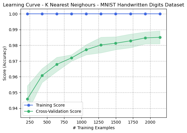
Figure 1: Learning Curve - K Nearest Neighbours - Digits Dataset
The timing curves for both datasets (Figs. 2, 3) show similar trends, which appear to indicate that fit times increase as a function of the number of training samples. Since the fit times of KNN should be ( O(1) ), a horizontal line was expected. These trends are possibly due to noise, computational randomness, or possibly include some data pre-processing steps in the KNN model generation. The tool used to generate these graphs was Scikit-Learn’s learning curve function.
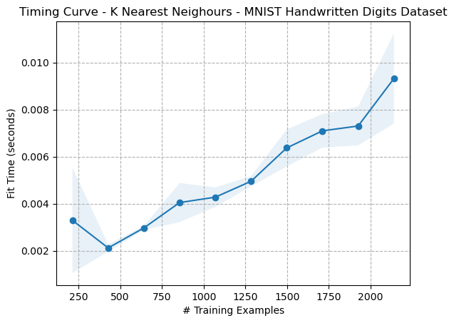
Figure 2: Timing Curve - K Nearest Neighbours - Digits Dataset
_KNearestNeighours_MNISTHandwrittenDigitsDataset.png)
Figure 3: Validation Curve (K) - K Nearest Neighbours - Digits Dataset
The most interesting hyperparameter to tune for KNN is, of course, K. With ( K=1 ), you are guaranteed to have a model with high bias that is susceptible to noise and overfitting. As K increases, a larger number of “nearest” neighbors are selected upon query, which can help generalize the model and prevent it from overfitting. This is seen in Figure 3. When ( K=1 ), the model actually performs best on unseen training data despite having the highest overall bias and variance. As K increases, the variance tends to decrease. This might be explained by the fact that the dataset is highly constrained to a strict data structure (individual, large pixels) that do not have a large degree of variation since it is only 8x8 pixels. One could hypothesize that a KNN learner would perform much more poorly on images with more pixels, where the digits could be written in a greater variety of locations or contexts. This is given the higher degree of variation and the necessary dependency on overall structure and patterns of the digits needed to properly classify, compared to the current example of comparing simple digit pixel intensities.
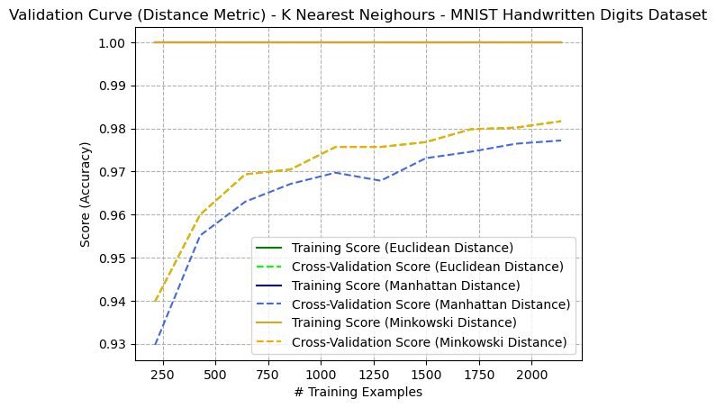
Figure 4: Validation Curve (Distance Metrics with K=5) - K Nearest Neighbours - Digits Dataset
The learning curves (validation curve) with ( K=5 ) of various distance metrics (Euclidean, Manhattan, and Minkowski) were compared in Figure 4. Note that the Euclidean lines matched the Minkowski lines perfectly, making it difficult to see them. This is because the Minkowski distance is a generalization of Euclidean and Manhattan distances. When the order ( p ) of the Minkowski distance is set to 2, it becomes the Euclidean distance. So, when ( p=2 ), the Minkowski distance and Euclidean distance will be the same. Thus, the only comparison became between Euclidean and Manhattan, where Euclidean performed best overall. This trend is similarly seen in Figure 8 on the Adult dataset.
Dataset 2: Adult Income Prediction
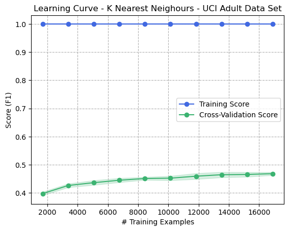
Figure 5: Learning Curve - K Nearest Neighbours - Adult Dataset
The learning curve (Fig. 5) for the Adult Income dataset demonstrates that KNN with ( K=1 ) performed dramatically worse than on the digits dataset. This is an example of a high bias, high variance model. Whereas the training set was predicted perfectly, the F1 score was below 0.5, showing very low precision and recall. There are many reasons why KNN might have performed poorly on this dataset. For example, it could be caused by non-uniformity in feature space: If the features of the data are not evenly distributed, then the distance metrics used by KNN may not be effective in finding the nearest neighbors. Additionally, this could mean that the dataset has a lot of outliers since KNN is highly sensitive to them. It can also perform poorly on imbalanced data.
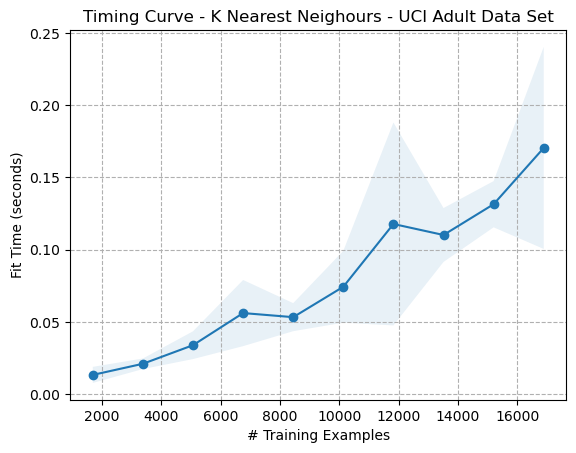
Figure 6: Timing Curve - K Nearest Neighbours - Adult Dataset
_KNearestNeighours_UCIAdultDataSet.png)
Figure 7: Validation Curve (K) - K Nearest Neighbours - Adult Dataset
The validation curve for altering K (Fig. 7) shows the effects of increasing K, causing a reduction in bias as well as a reduction in variance. Unfortunately, the low-bias, low-variance model performs more poorly on unseen data than the high bias, high variance model (( K=1 )).
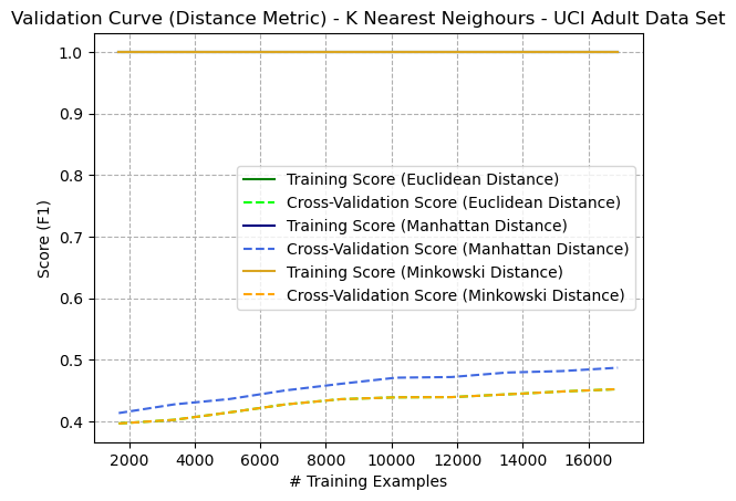
Figure 8: Learning Curve (Distance Metric with K=5) - K Nearest Neighbours - Adult Dataset
Support Vector Machines
Dataset 1: Digits
| Kernel Type | Poly (degree 3) |
|---|---|
| Regularization Param C | 1 |
Table: Hyperparameter Values - SVM - Digits Dataset
For all results excluding the Kernel validation curves, the SVM was trained using the hyperparameters indicated in the table above.
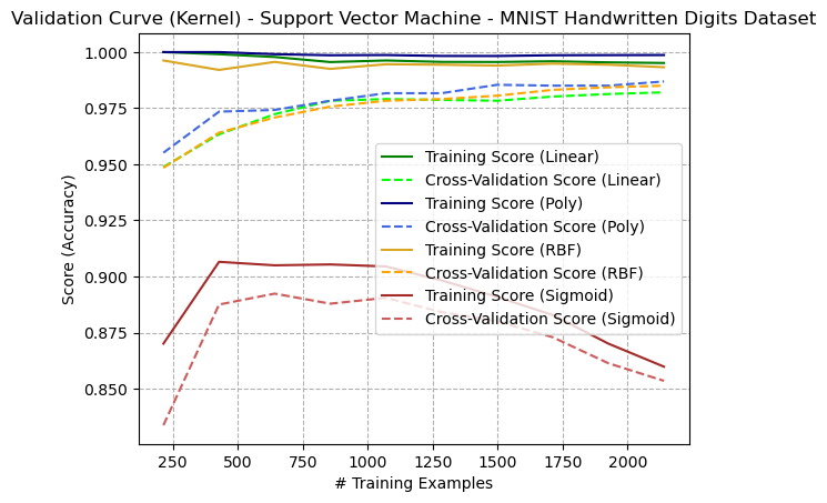
For Support Vector Machines, the most interesting hyperparameter to study is the kernel function. The kernel function transforms the input data into a higher dimensional space to make it linearly separable, and the choice of kernel is important for the functionality of the SVM and can also depend on the type of data being used. In the figure above, the learning curves of four different kernels are shown. The kernels are:
- Linear: Uses a simple linear transformation and is best suited for linearly separable data.
- Polynomial: For data that is not linearly separable; the degree of the polynomial determines the model’s complexity.
- Radial Basis Function (RBF): A function that has a value of 1 at the origin and decreases away from the origin, and can model both linear and non-linear patterns.
- Sigmoid: Similar to the RBF kernel.
The training curves indicate that all three of the Linear, Poly, and RBF kernels perform well at generating relatively low variance, high accuracy models. The polynomial model appears to have a high bias that does not decrease with increased training examples, possibly indicating overfitting. The fact that the linear kernel was successful indicates that the data is likely linearly separable. It is interesting that the Sigmoid kernel performed poorly on the dataset. This could be because it’s a non-linear function and is designed to capture non-linear relationships in the data. When a sigmoid kernel is applied to a linearly separable dataset, it may create a more complex model that fits the data poorly, potentially leading to overfitting.
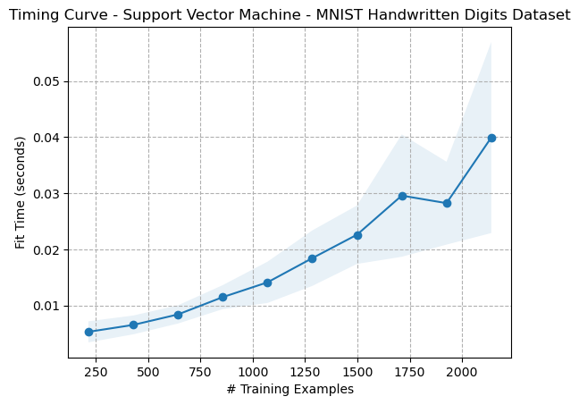
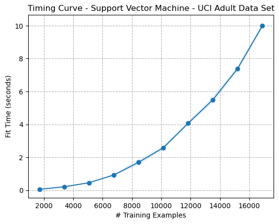
The timing curves in the figures above are interesting because they appear to align with the 3rd order polynomial kernel used for their transformation. The time complexity of a polynomial kernel on an SVM for fitting data is (O(n^d)), where n is the number of training samples and d is the degree of the polynomial kernel.
_SupportVectorMachine_MNISTHandwrittenDigitsDataset.png)
The regularization parameter helps determine the trade-off between getting a low training error and a low testing error, balancing overfitting and underfitting. A smaller value of C allows for a larger margin for the decision boundary, which results in more misclassified samples but can reduce overfitting. Conversely, a larger value of C results in a smaller margin, potentially leading to overfitting. In the figures above, it can be seen that increasing the value of C increases the bias toward training data (overfitting).
Dataset 2: Adult Income Prediction
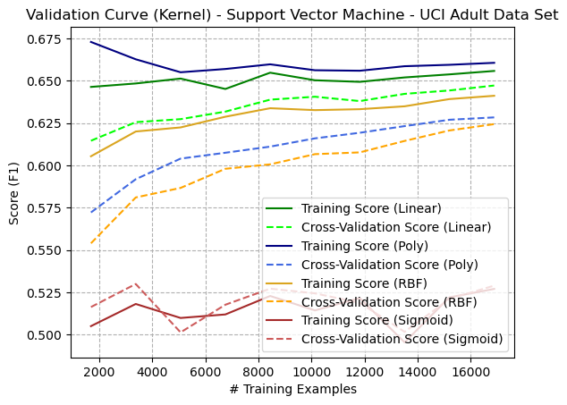
Similar to the Digits dataset, the Polynomial kernel performed best on the Adult dataset, but only on the training set. The linear kernel performed best overall when considering the cross-validation score, indicating that the polynomial kernel had overfit the training data, leading to higher bias and variance.
_SupportVectorMachine_UCIAdultDataSet.png)
This conversion maintains the structure and details of the original LaTeX code, with images and tables formatted to fit markdown syntax.
Neural Networks
Dataset 1: Digits
Hyperparameters - ANN
| Hyperparameter | Value |
|---|---|
| Hidden Layer Size | (64) |
| Alpha | 0.00005 |
| Activation | Relu |
Table: Hyperparameter Values - ANN - Digits and Adult Dataset
For both datasets, the hyperparameters were as per Table {annt1}, with the exception of hidden layer sizes. For the Digits dataset, the hidden layer size was (64) to correspond with the 64 input features. For the Adult dataset, the hidden layer size was (52, 26, 26, 26). The 52 corresponded with the number of features after one-hot encoding had expanded the number of rows.
Learning (Validation) Curve - Digits Dataset
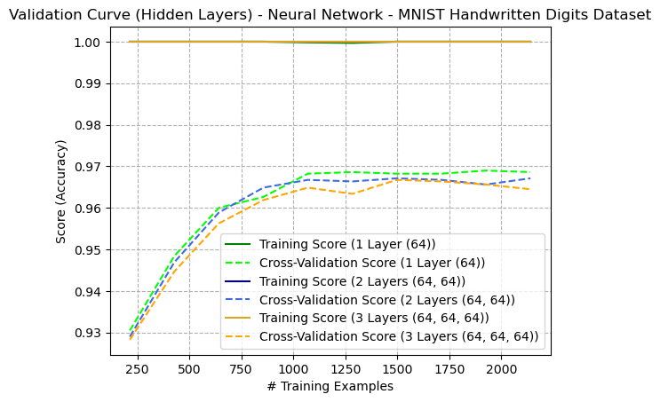 Figure: Learning Curve (Number of Hidden Layers) - Artificial Neural Network - Digits Dataset (Figure {ann4})
The learning curve showing different hidden layer sizes for the Digits Dataset reveals that additional hidden layers did not contribute to overall performance. This may indicate that the dataset is not complex enough to merit additional layers and can be classified with a linear model. This is likely the case, since the digits inputs are simplified (only an 8x8 image). One might hypothesize that a higher number of hidden layers would be appropriate for classifying more complex images of digits, such as images with higher dimensionality. In all cases, the learners appeared to overfit the training data.
Iterative Learning Curve - Digits Dataset
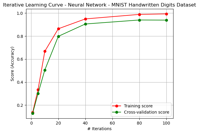 Figure: Iterative Learning Curve - Artificial Neural Network - Digits Dataset (Figure {ann1-2})
The iterative learning curve (Figure {ann1-2}) shows the effect of epochs on performance. The model tended to overfit training data, but the variance remained constant, with convergence occurring at around 100 iterations.
Timing Curve - Digits Dataset
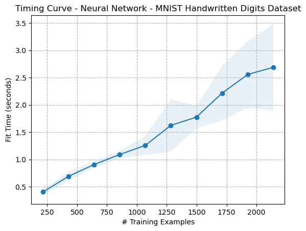 Figure: Timing Curve - Artificial Neural Network - Digits Dataset (Figure {ann2})
The timing curve (Figure {ann2}) shows a linear relationship between the number of training examples and fit time. The time complexity of fitting an ANN is ( O(n*m) ), where ( n ) is the number of examples and ( m ) is the number of parameters in the model \cite{coates2011analysis}. By parameters, this means the number of weights in the model. The output appears to match this.
Validation Curve (Learning Rate Alpha) - Digits Dataset
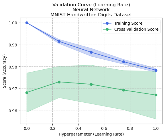 Figure: Validation Curve (Learning Rate Alpha) - Artificial Neural Network - Digits Dataset (Figure {ann3})
The validation curve (altering alpha) was conducted to see how it would impact performance. With a very small alpha, the speed of convergence is much slower. However, the ability of the model to conform closely to input data increases, thus causing overfitting. Figure {ann3} demonstrates this behavior, where the model overfits with small alpha but creates a more generalized model as the alpha increases to about 0.2. However, as the alpha increases up to 1, it is possible that the global maximum is not found, and both the training and cross-validation scores begin to drop. This could be caused by a lack of convergence due to overcompensation in weight updates during the backpropagation step.
Dataset 2: Adult Income Prediction
Learning (Validation) Curve - Adult Dataset
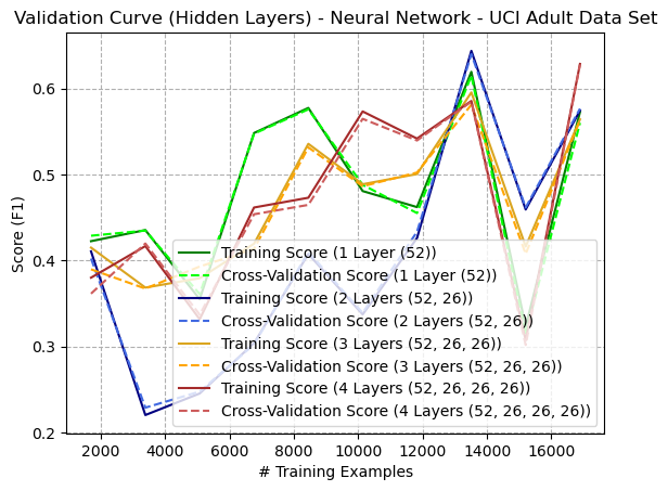 Figure: Learning (Validation) Curve (Number of Hidden Layers) - Artificial Neural Network - Adult Dataset (Figure {ann8})
The learning/validation curve for the Adult dataset (Figure {ann8}) is interesting because it produces oscillating performance based on the number of training examples. In particular, all models seemed to drop substantially in performance at around 15,000 samples. This is difficult to explain but could be due to several factors. Some factors include overfitting, which could mean that adding more training examples may not necessarily improve performance on unseen data; in fact, it could worsen the overfitting problem, causing the model to perform worse on the validation set. Another factor could be model complexity: if the model is too complex for the size of the training set, the high number of parameters (weights) relative to the number of examples could cause it to fit the noise in the data rather than the underlying patterns. The data samples up until that point could also be non-representative of the whole dataset. The dataset being imbalanced could cause the model to try to predict the majority class most of the time.
Iterative Learning Curve - Adult Dataset
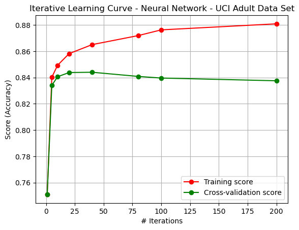 Figure: Iterative Learning Curve - Artificial Neural Network - Adult Dataset (Figure {ann5_2})
The iterative learning curve (Figure {ann5_2}) shows that increased iterations actually caused overfitting to the training data (increased bias and variance), thus performing worse on unseen data.
Timing Curve - Adult Dataset
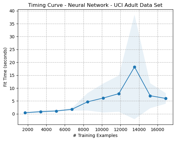 Figure: Timing Curve - Artificial Neural Network - Adult Dataset (Figure {ann6})
A similar trend is seen in the validation curve (Figure {ann7}), whereby the increased value of alpha causes a degradation in performance, as the model is incapable of fitting the training data effectively, possibly from non-convergence or being incapable of finding a global maximum.
Validation Curve (Learning Rate Alpha) - Adult Dataset
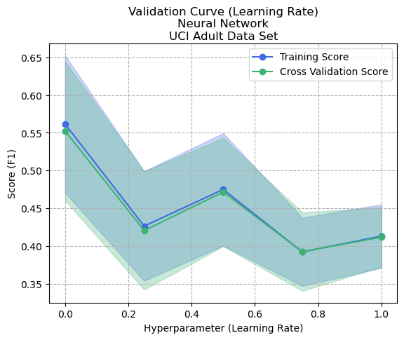 Figure: Validation Curve (Learning Rate Alpha) - Artificial Neural Network - Adult Dataset (Figure {ann7})
Overall Comparison
Performance Comparison
Digits Dataset
| Learner | Fit Time (s) | Predict Time (s) | Accuracy | F1 Score |
|---|---|---|---|---|
| Decision Tree | 0.020 | 0.001 | 0.886 | 0.886 |
| Boosting | 3.490 | 0.110 | 0.920 | 0.923 |
| KNN | 0.009 | 0.185 | 0.985 | 0.985 |
| SVM | 0.059 | 0.030 | 0.840 | 0.842 |
| ANN | 2.050 | 0.013 | 0.950 | 0.950 |
Table: Performance Results - Digits Dataset (Table {comparison_digits})
Adult Dataset
| Learner | Fit Time (s) | Predict Time (s) | Accuracy | F1 Score |
|---|---|---|---|---|
| Decision Tree | 0.060 | 0.002 | 0.857 | 0.850 |
| Boosting | 11.900 | 0.680 | 0.866 | 0.862 |
| KNN | 0.145 | 13.200 | 0.775 | 0.759 |
| SVM | 16.980 | 2.480 | 0.769 | 0.768 |
| ANN | 28.520 | 0.010 | 0.833 | 0.820 |
Table: Performance Results - Adult Dataset (Table {comparison_adult})
Throughout this report, various algorithms were applied with different hyperparameters across two datasets. Training, validation, and timing curves were collected for each. Tables {comparison_digits} and {comparison_adult} summarize the results, showing the final performance metrics based on the learners’ application against the test data. Several notable differences between algorithms can be analyzed:
-
F1 Score Discrepancies: The F1 Scores for the Adult Dataset (Table {comparison_adult}) were considerably better than the cross-validation scores. This could be due to the larger total training data used for the final models compared to the K-Fold split during cross-validation.
-
Decision Trees: Decision Trees are fast in both training and prediction times and are straightforward to understand. They performed well on both datasets but were prone to overfitting when allowed to grow too complex. This might explain their good performance on the Digits Dataset compared to the MNIST dataset.
-
Boosting: Boosting with Decision Tree (DT) Weak Learners was robust against overfitting and provided similar or better performance compared to Decision Trees, though at the cost of increased fit and predict times (which increase with the number of weak learners). Decision Trees are sometimes considered ideal for small, well-defined datasets, which may explain their effectiveness on the Digits Dataset.
-
KNN: KNN algorithms are simple and can be trained in (O(1)) time, assuming the dataset fits in memory. With (K=1), KNN models performed well on the Digits Dataset due to its simplicity but struggled with the Adult Dataset due to noise and complexity. The susceptibility to noise in KNN models with (K=1) explains the variation in performance.
-
Support Vector Machines (SVM): SVMs, using different kernels, minimize overfitting by maximizing the margin between classified samples and can handle both linear and non-linear data. Despite their effectiveness in theory, SVMs performed poorly overall in these datasets, with particularly high fit times, especially with a polynomial kernel.
-
Artificial Neural Networks (ANN): ANNs excel with complex, non-linear data. Although the first dataset was somewhat linear, the ANN performed acceptably with a single hidden layer. The ANN showed the largest fit times but the shortest predict times, and performed well on the Adult Dataset.
References
-
Deng, L. (2012). The MNIST Database of Handwritten Digit Images for Machine Learning Research. IEEE Signal Processing Magazine, 29(6), 141-142. Link. ↩
-
Kohavi, R., & Becker, B. (1996). UCI Adult Dataset - Machine Learning Repository. Data Mining and Visualization, Silicon Graphics, Inc. Link. ↩
-
Freund, Y., & Schapire, R. E. (1997). A Decision-Theoretic Generalization of On-Line Learning and an Application to Boosting. Journal of Computer and System Sciences, 55(1), 119-139. Link. ↩
-
Bühlmann, P., & Hothorn, T. (2007). Boosting Algorithms: Regularization, Prediction, and Model Fitting. Statistical Science, 22(4), 477-505. Link. ↩
-
Cormen, T. H., Leiserson, C. E., Rivest, R. L., & Stein, C. (2001). Introduction to Algorithms. MIT Press. ↩


Comments