
Randomized Optimization Algorithms: An Exploration

Randomized Optimization - An Exploration
Evan Loughlin
Index Terms machine learning, randomized optimization, hill climbing, simulated annealing, genetic algorithms, MIMIC
I. Introduction
Randomized optimization algorithms use randomized search heuristics to find approximate solutions to optimization problems. In this study, we present an analysis of four randomized optimization algorithms: Randomized Hill Climbing, Simulated Annealing, Genetic Algorithms, and MIMIC. The goal is to explore the strengths and limitations of each algorithm and to investigate their performance across three problems: Graph Coloring, Knapsack Problem, and the N-Queens Problem. Specifically, the aim is to highlight the characteristics of the problems that make them better suited to a particular algorithm, shedding light on the underlying mechanisms that enable each algorithm to excel at certain types of problems.
In addition, the analysis is extended to the domain of neural network optimization, where we apply the first three randomized optimization algorithms to find optimal weights in an existing neural network, whereby results are compared and analyzed against using standard back propagation.
II. Methods
In this project, 4 different Randomized Optimization algorithms were studied: Randomized Hill Climbing, Simulated Annealing, Genetic Algorithms, and MIMIC. Three problems were selected: Graph Coloring, Knapsack Problem, and the N-Queens Problem.
In Part 1, experiments were run for each algorithm on each problem to collect data regarding their performance. This data includes how many function evaluations are performed per iteration, wall clock time per iteration, and fitness score per iteration. Furthermore, hyperparameters of each of the algorithms’ were modified in order to study their effects solving problems. In Part 2, an existing neural network’s weights are optimized using the first three listed algorithms, and performance is compared to the original backpropagation algorithm. The implementation of algorithms and problems discussed in this experiment utilized mlrose - hiive package [4], in addition to Jupyter Notebooks to run experiments.
III. Problems
A. Graph Coloring Problem
The Graph Coloring problem [10]: Given a graph and some limited number of colors, the goal of this problem is to color each node of the graph in a way such that no two adjacent nodes have the same color. The time complexity of the Graph Coloring problem is exponential with O(Dn), where D is the maximum degree of the graph and n is the number of nodes in the graph.
This problem was selected in order to highlight the benefits of the MIMIC algorithm, because the problem is known to have a large degree of dependency between variables, and MIMIC is able to capture dependencies between variables more effectively than other algorithms [2]. This is because MIMIC uses a probabilistic model to estimate the joint distribution of the variables, and therefore is able to capture dependencies between variables that other algorithms may not notice.
B. Knapsack Problem
The Knapsack Problem [6]: Given a set of items (such as gems), each with their own weight and value, and a knapsack with a maximum weight capacity, the goal of this problem is to determine the optimal combination of items to include in the knapsack such that the total weight is less than or equal to the maximum capacity, and the total value is maximized. The time complexity of the Knapsack problem is also exponential, O(2n), where n is the number of items.
This problem was selected to highlight the benefits of the Genetic Algorithm. The GA is well suited to problems with discrete decision variables, since it uses crossover and mutation techniques to explore a large search space, and is able to handle multiple optimal solutions. Unlike the Graph Coloring problem, variables have fewer dependencies and the state of each possible state is relatively loosely constrained (no dependencies between variables), given that the Knapsack problem only has a single constraint (that total weight not be exceeded).
C. N-Queens Problem
The N-Queens Problem [1] involves placing N chess queens on a chess board of dimensions N x N, such that no two queens are attacking one another (queens can attack horizontally, vertically, and diagonally).
The N-Queens problem is considered to be NP-Hard, and has complexity of O(n!), making it infeasible to search exhaustively through the solution space. For example, a 20-queens problem has over 39 quintillion possible solutions. It is therefore a fantastic candidate for randomized optimization problems.
Simulated annealing is hypothesized to be a good algorithm for solving this problem, since it is able to immediately start searching over a large search space efficiently, and can escape local optima more easily than other algorithms [7]. In the N-Queens problem, local optima occur when a particular configuration of queens is stuck in a position where they cannot move without violating the chess constraints.
D. Problem Sizes
For each of these problems, 3 different versions were implemented (called small, medium, and large sizes), in order to assess how the size of the problem can impact the performance of each algorithm. Table I describes the size of each problem implemented. For N-Queens, N is the dimension of the board and number of Queens to place. For Graph Coloring, N is the number of nodes (for each problem, number of colours = 3). For the Knapsack problem, N is the number of items (or gems) that can be selected to fill the bag. The max weight of the bag was selected to always be 50% of the total weight of all items.
| Problem | Small | Medium | Large |
|---|---|---|---|
| N-Queens | N = 5 | N = 10 | N = 20 |
| Graph Coloring | N = 5 | N = 10 | N = 20 |
| Knapsack | N = 10 | N = 50 | N = 100 |
TABLE I
Problem Sizes
IV. Part 1: Randomized Optimization
A. Randomized Hill Climbing
Randomized Hill Climbing (RHC) was run on each of the problems, and acts as a baseline from which to compare the other algorithms. RHC starts with a random initial solution and then iteratively improves the solution by creating new candidate solutions [8] which are in close proximity (thus “climbing” up the hill to a maxima). The randomized aspect derives from the fact that the next candidate is selected randomly from a set of possible candidates, which can help the algorithm avoid getting stuck in local optima.
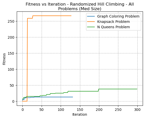
Fig. 1. Fitness VS Iteration - Randomized Hill Climbing - All Problems (Med Size)
In Fig 1, it’s clear to see that the algorithm converged quickly for the Knapsack and Graph Colouring Problem, but slowly for the N-Queens problem. An important note on all graphs comparing fitness in the Y-Axis: each problem (and each size of problem) would have its own unique maximum fitness. It’s therefore not possible with these graphs to know if the algorithm has found a global maxima or a local maxima. Therefore, with these types of graphs we’re primarily just considering the rate of convergence. In this particular graph, the N-Queens slowly converged. This may be due to the N-Queens problam having more a discrete and jagged fitness landscape with many local optima. The Knapsack problem, for example, has a more continous and smoother fitness landscape that may make it more suitable.
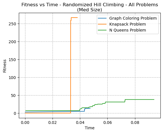
Fig. 2. Fitness VS Time - Randomized Hill Climbing - All Problems (Med Size)
The Fitness versus Time graph (Fig 2) shows a similar trend, with the knapsack problem rapidly converging.
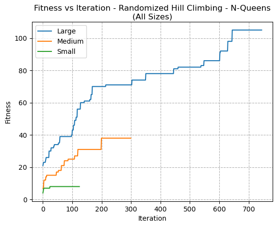
Fig. 3. Fitness VS Iteration - Randomized Hill Climbing - N-Queens (All Sizes)
In order to analyze more closely how the size of problem impacts the performance, 3 sizes of the N-Queens problem was compared in Fig 3. It can be seen how the RHC makes gradual improvements toward a goal without ever appearing to decrease in fitness from one iteration to the next. The behaviour seems consistent for all problem sizes.
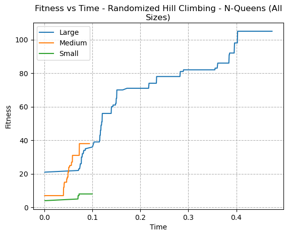
Fig. 4. Fitness VS Time - Randomized Hill Climbing N-Queens (All Sizes)
Since RHC explores neighbours with randomness, this helps it escape local optima. In general, RHC evaluates the objective function once per iteration to determine whether the next possible solution is an improvement. If the next solution is not, RHC would discard it and generate a new candidate. Fig 23 shows that this trend is correct, since the plot of the line of function evaluations per iteration is straight.
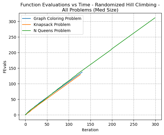
Fig. 5. Function Evaluations VS Time - Randomized Hill Climbing - All Problems (Med Size)
B. Simulated Annealing
Simulated annealing (SA) was run on each of the problems, and a comparison of the medium size problems’ fitness convergence is seen in Fig 6. For this graph, a Temperature of 1.0 is used. Similar to RHC, SA performed very well on the Knapsack problem, converging to a solution very quickly. In fact, SA behaved relatively similarly to RHC. Some key difference between the algorithms, however, is that SA has the concept of temperature which allows it to more rapidly explore the solution space than RHC. This also makes it possible for SA to temporarily accept worse solutions in the search for a global optimum.
The similarity between behaviour of SA and RHC might be explained because of low temperature. When temperature is sufficiently low, the SA algorithm is less likely to make large jumps in the solution space and would therefore behave more similary to RHC.
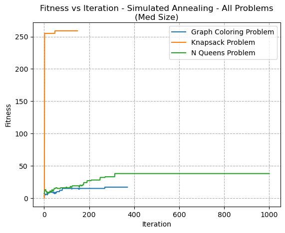
Fig. 6. Fitness VS Iteration - Simulated Annealing - All Problems (Med Size)
This trend can be visualized when reviewing Fig 7, where the medium size Graph Coloring Problem was used and the temperature was increased. As temperature increases, the fitness score oscillates. This is because the algorithm can accept worse solutions, and can make larger jumps in the solution space. When temperature is set too high, the search becomes more random and ineffective, as the algorithm would move to any random solution regardless of the change in the objective function. This is because the probability of accepting a worse solution approaches 1 as temperature increases. [9]

Fig. 7. Fitness VS Iteration - Simulated Annealing - Graph Coloring Problem (Med Size) - ExpDecay - Tuning Temperature
Decay type was also tuned, and can be seen in Fig 8. The decay type decides how the temperature decreases with iteration. The graph shows that the behaviour of fitness is very similar, although the ExpDecay appears to decrease temperature more rapidly.
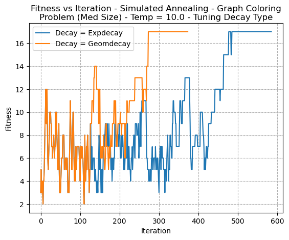
Fig. 8. Fitness VS Iteration - Simulated Annealing - Graph Coloring Problem (Med Size) - Temp=100 - Tuning Decay Type
The fitness vs time graph was computed 9 to demonstrate the relative speed by which convergence was found for each of the three problems. In this case, both the Knapsack and Graph Coloring problems appeared to converge quickly. However, it’s notable that the final solution for the knapsack problem has a visually lower fitness than on a previous iteration, likely due to afforementioned temperature affects.

Fig. 9. Fitness VS Time Simulated Annealing - All Problems (Med Size) Temp=10.0 ExpDecay
SA made more function evaluations than simply one per iteration, as per 10, as the slope of the line is clearly non-linear. By making multiple evaluations per iteration, the algorithm can explore the search space more efficiently and converge faster.

Fig. 10. Function Evaluations VS Iteration - Simulated Annealing - All Problems Med Sizes Temp=100 ExpDecay
C. Genetic Algorithms
The Genetic Algorithm appeared to show a smooth continuous convergence for each of the problems (Fig 11). This is because of how they work. They use a population of solutions that undergo a process of selection (based on best fitness), crossover (breeding) and mutation (like how DNA mutates), such that there is a survival of the fittest concept.
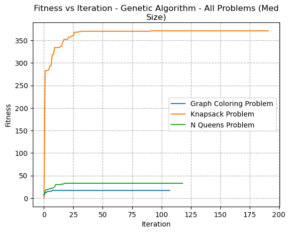
Fig. 11. Fitness VS Iteration - Genetic Algorithm - All Problems (Med Size)
For different sizes of problems, the GA appeared to converge more quickly for smaller problems, although displayed similar patterns in its convergence (Fig 12).
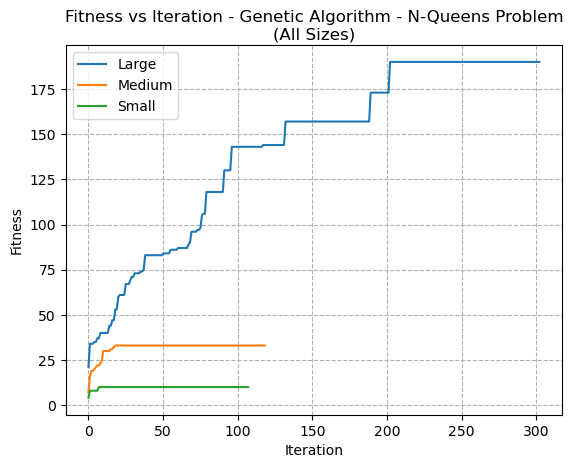
Fig. 12. Fitness VS Iteration - Genetic Algorithm - N-Queens Problem (All Sizes)
The mutation rate is what controls much of the randomness of the algorithm, and is what can allow it to explore more of the solution space. If the mutation rate is set too low, this can result in the algorithm getting stuck in a local optimum and not being able to escape to find the global optimum. An example of this is shown in figure 13, where Mutation Rate = 0.1 converges to a lower fitness score than with Mutation Rate = 0.3, despite it being the same problem.
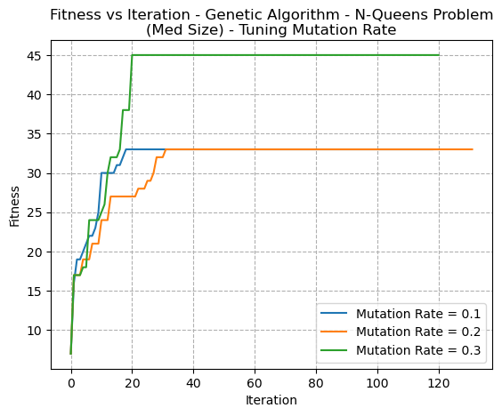
Fig. 13. Fitness VS Iteration - Genetic Algorithm - N-Queens Problem (Med Size) - Tuning MutationRate
Although the GA is known to perform well on problems like the Knapsack problem [3], these graphs intentionally focus on its performance on the N-Queens problem in order to demonstrate how the N-Queens problem has many local optima, and by reducing the mutation rate (or any algorithm’s ability to randomly explore the solution space), it can fall into local optima. Furthermore, the solution space of the N-Queens problem is highly constrained, therefore many of the potential solutions are infeasible thus limiting the search space for the genetic algorithm.
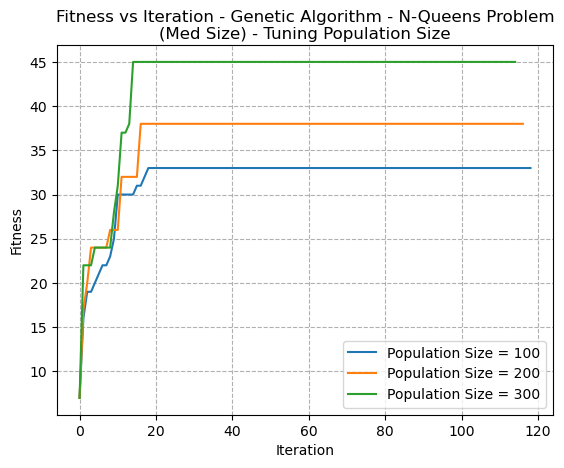
Fig. 14. Fitness VS Iteration - Genetic Algorithm - N-Queens Problem (Med Size) - Tuning Population Size
Tuning was also conducted on the crossover rate, as well as the population size. For these problems, the crossover rate didn’t greatly impact the convergence rate or fitness score. However, larger population sizes allowed the algorithm to more quickly explore larger random reaches of the search space. It was also found that when the mutation rate is too high, analogous to SA’s temperature, the search can become too random and fail to converge to an optimal solution. Instead, the population may continue to mutate and diverge, resulting in a loss of good solutions and a lack of progress towards an optimal solution.
D. MIMIC
MIMIC is a probabilistic optimization algorithm that uses a model-based approach, order to search large spaces for optimal solutions, and is well-suited for problems with a high degree of dependencies among variables.
In the graph coloring problem, each node in the graph represents a variable that can take on a specific color. The dependencies arise from the fact that the color assigned to a vertex can depend on the colors assigned to its neighbouring vertices. This means that the choice of one colour affects the choices available for another.
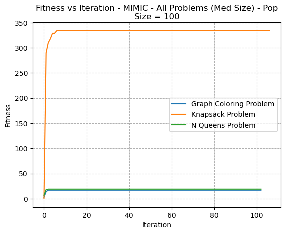
Fig. 15. Fitness VS Iteration - MIMIC All Problems (Med Size) PopSize=100
In figure 15, a very rapid convergence pattern is seen for all three problems. Whether these are local or global optima can not be ascertained from this image. However, the same type of pattern is seen when reviewing different sizes of the same problem. (Fig 16)
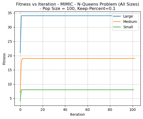
Fig. 16. Fitness VS Iteration - MIMIC N-Queens Problem (All Sizes) PopSize=100- KeepPercent=0.1
In figures 17 and 18, the hyperparameters of Keep Percentage and Population Size are respectively tuned. In both cases, as they parameters increase, there’s a higher convergence. This indicates that this helps the algorithm escape from local optima by exploring a larger amount of the search space. This is similar to what was discussed with SA (temperature) and GA (mutation rate and population sizes). It should be noted that increased randomness (searching more space by increasing the population size and the keep percentage) could result in a slower run time, since greater amounts of possible solutions need to be assessed at each iteration.
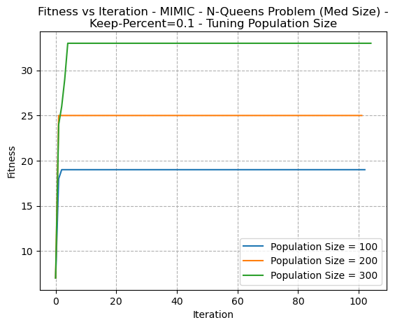
Fig. 17. Fitness VS Iteration - MIMIC N-Queens Problem (Med Size)- KeepPercent=0.1 - Tuning Population Size
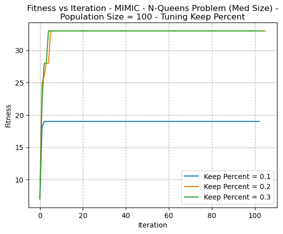
Fig. 18. Fitness VS Iteration - MIMIC N-Queens Problem (Med Size) Population Size 100 - Tuning Keep Percent
It can be seen that for MIMIC, a constant (proportional to population size) number of function evaluations are required at each iteration, as can be seen in Fig 19.
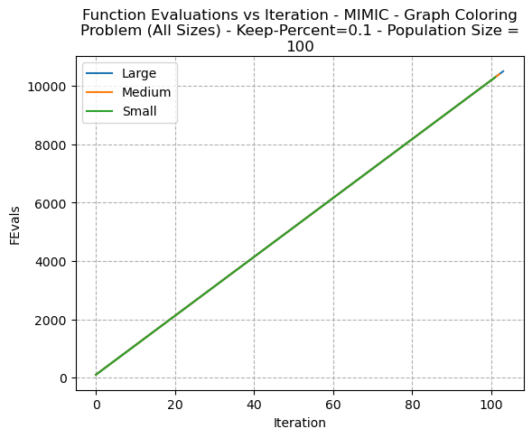
Fig. 19. Function Evaluations VS Iteration MIMIC Graph Coloring Problem - (All Sizes)- KeepPercent=0.1 Population Size 100
V. Overall Comparison
An overall comparison of problems was completed for each of the Medium sized problems. For the Graph Coloring Problem (Fig 20), the MIMIC algorithm performed very well, with fewer iterations. It should be noted, however, that the MIMIC algorithm performs more function evaluations per iteration, as previously discussed. Interestingly, the genetic algorithm also performed well. It might be speculated that larger problem sizes would elicit greater divergences in algorithm performance. The RHC algorithm failed to find the same optimum values as the other three algorithms, and settled in a local optima. The SA algorithm took many more iterations, and oscillated (due to temperature), but eventually found the same solution as GA and MIMIC.
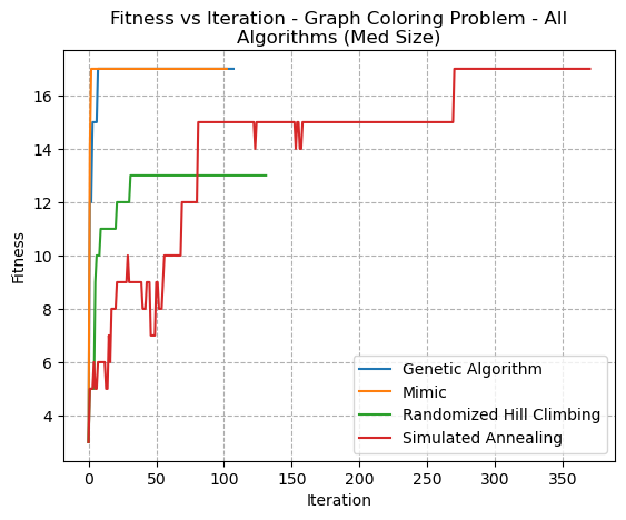
Fig. 20. Fitness VS Iteration - Graph Coloring Problem - All Algorithms(Med Size)
The Knapsack problem (Fig 21) showed interesting differences between each of the algorithms, and demonstrated how the GA excels at such problems. The GA performed best, followed by MIMIC. Both SA and RHC settled into local optima at much lower fitness values. This is because the GA excels at handling large spaces with many possible solutions.
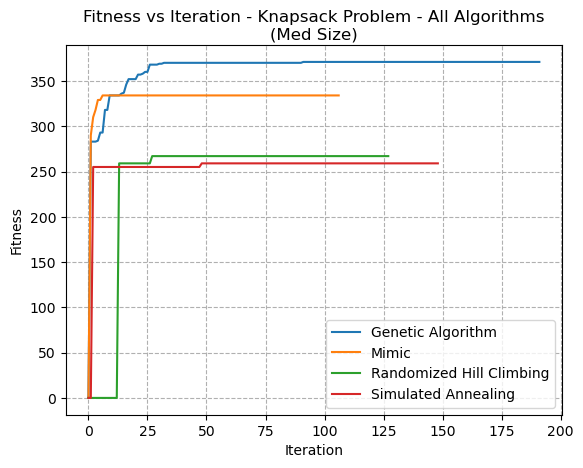
Fig. 21. Fitness VS Iteration - Knapsack Problem - All Algorithms(Med Size)
The N-Queens problem overall (Fig 22) showed marked differences between the algorithm’s performances. The MIMIC algorithm did poorest. This may be because, although the N-Queens problems has tight constraints on the placement of queens, each variable (queen) can be placed independent of the others, and the objective function depends only on the placement of the queens. Therefore, MIMIC may not be able to take advantage of dependencies among the variables. This could explain why algorithms that do not depend on the joint distribution among variables, such as GA, SA, and RHC, might perform better. Simulated Annealing and RHC performed best. As discussed previously, when temperature is low, SA behaves similarly to RHC. It did well because it can escape from local optima. The N-Queens problem has many local optima, and random restart algorithms liek GA might get stuck in them. SA uses probabilistic distributions to determine whether to accept or reject candidate solutions, and additionally allows for ”bad” moves to be made which can help it roll out of local optima.
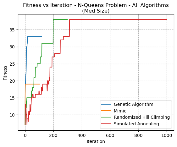
Fig. 22. Fitness VS Iteration - N-Queens Problem - All Algorithms(Med Size)
VI. Part 2: Neural Network Backpropagation Comparison
A. Introduction
In Assignment 1: Supervised Learning, a neural network was trained for a particular dataset. The dataset under consideration is the UCI Adult Dataset [5]. Hyperparemeters were tuned via grid search. The resulting neural network trained for this consisted of layers of the form (56, 23, 23), and an activation function of relu. The alpha for this network was 0.00005. Figure 23 shows the results of the cross-validation curve per iteration of the backpropagation algorithm for the ANN. The figure demonstrates the algorithm’s gradual improvement as iterations began, leading to in increase in variance as iterations became large, thus leading to overfitting to training data.
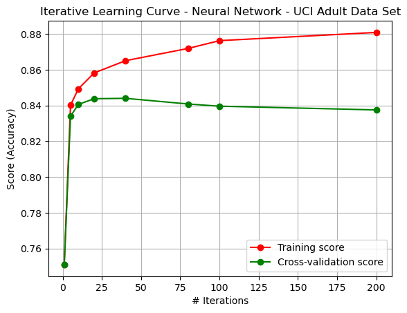
Fig. 23. Iterative Learning Curve - Backpropagation
In order to assess the performance of the Genetic Algorithm, Simulated Annealing, and Randomized Hill Climbing on their ability to optimize weights for the neural network, the mlrose NNGSRunner function was run. The learning rate was specified here as 0.1. Most of the problems were found to be computationally intensive, thus number of iterations was limited to 100 for each algorithm.
It’s important to note that in mlrose, the metric used to evaluate the performance of the neural network is the mean squared error (MSE). The Fitness score is used to compare different combinations of hyperparameters and select the best performing combination. The best combination of hyperparameters is the one that achieves the highest Fitness score on the evaluation dataset.
Note that the Fitness score returned by the NNGSRunner is not the same as the fitness score used in optimization problems. In optimization problems, the fitness score is a measure of how well a particular solution (i.e., a set of parameters) performs on the objective function being optimized. In the context of the NNGSRunner, the Fitness score is a measure of how well the neural network performs on the evaluation dataset, given a set of hyperparameters. In reviewing
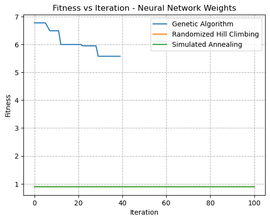
Fig. 24. Fitness VS Iteration - Neural Network Weight Optimization
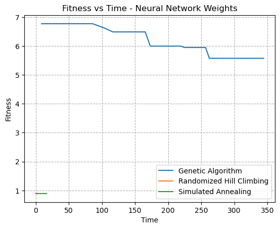
Fig. 25. Fitness VS Time - Neural Network Weight Optimization
For both of Figs 24 and 25, the Simulated Annealing problem and the Randomized Hill Climbing problems failed to find improvements over the current weights. In these graphs, what’s shown as the fitness is the overall loss, and thus decreasing loss leads to greater overall performance. It should be noted howevever that a limited amount of hyperparameter tuning was completed. Although, it may be concievable that a higher degree of randomness introduced into either the SA algorithm or the RHC algorithm could help candidate solutions escape local optima. The failure to find convergence may be for a number of reasons. For one, they could have pre-maturely converged to a suboptimal solution, and have been stuck in local optima. The large number of weights (52) in the problem could also contribute to a lack of benefit, and thus a lack of change in any direction.
Additionally, the weights in Neural Networks are not discrete values as were analyzed in the previous section. This means that randomized optimization would need to know by how much a value should be tweaked. For discrete problems, it’s easy to simply switch an element or bit. However, real numbers are uncountably infinite, and the knowledge of how much of a change in weights would be crucial. It could be possible that the change in weights was far too small to see a difference, or so large that the performance was consistently poor and too random to converge.
This dataset is also known to contain a considerable amount of noise. Noise in the data could also contribute to difficulties in finding convergence.
The Genetic Algorithm, on the other hand, did appear to find gradual improvements in the overall performance of the weights. This could be because they’re effective at finding global optima, in particular for problems where variables have loose coupling. They’re also good at managing noisy or incomplete data. It seems feasible that the genetic algorithm would be better suited for optimization of weights
The overall comparison of performance between different algorithms in terms of the overall performance of the Neural Network on predicting the class of the Adult Dataset is seen in the table below.
| Algorithm | Accuracy |
| Backpropagation | 0.769 |
| Genetic Algorithm | 0.743 |
| Simulated Annealing | 0.467 |
| Random Hill Climbing | 0.465 |
A closer examination of the fitness scores based on several different runs with varying hyperparameters was performed to see how the fitness changed by iteration. Figs 26, 27, and 28 show the Fitness versus Iteration curves for multiple runs of the Randomized Hill Climbing, Simulated Annealing, and Genetic Algorithms, respectively.
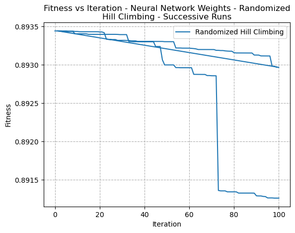
Fig. 26. Fitness VS Time - Neural Network Weight Optimization - Randomized Hill Climbing
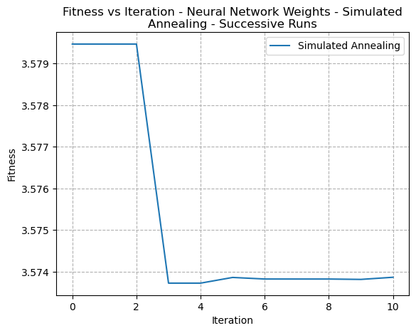
Fig. 27. Fitness VS Time - Neural Network Weight Optimization - Simulated Annealing
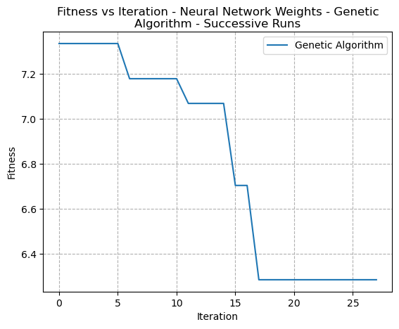
Fig. 28. Fitness VS Time - Neural Network Weight Optimization - Genetic Algorithms
In these closer graphs, it’s clear to see that both the Simulated Annealing algorithm as well as the RHC algorithms did appear to make incremental improvements in reduction of error. It may the case however that step size needed to be increased in order to improve the speed of convergence.
VII. Summary
In conclusion, the study provides a comprehensive analysis of four randomized optimization algorithms and their performance on three different optimization problems. The analysis reveals that each algorithm has its strengths and limitations and is well-suited for solving specific types of problems. The study highlights the importance of choosing the appropriate algorithm for a given problem, based on the problem’s characteristics and constraints. The study also extends its analysis to the domain of neural network optimization, demonstrating that randomized optimization algorithms can be effective alternatives to standard backpropagation algorithms. Overall, the study contributes to the understanding of randomized optimization algorithms and provides valuable insights for solving a wide range of optimization problems.
References
[1] Ian H Bell. The n-queens problem: an introduction to combinatorial search. Contemporary Physics, 50(4):423–434, 2009.
[2] Jeremy S De Bonet, Charles L Isbell, and Paul A Viola. Mimic: Finding optima by estimating probability distributions. In Advances in neural information processing systems, pages 424–430, 1999.
[3] John J Grefenstette. Optimization of control parameters for genetic algorithms. IEEE Transactions on Systems, Man, and Cybernetics, 16(1):122–128, 1985.
[4] Max Halford and Hiive. mlrose-hiive: Machine learning, randomized optimization, and search package. https://github.com/hiive/mlrose, 2022.
[5] Ronny Kohavi and Barry Becker. UCI adult dataset - machine learning repository, 1996.
[6] Silvano Martello and Paolo Toth. The knapsack problem: 1. definitions and relations to other problems. Surveys in Operations Research and Management Science, 2(3):163–197, 1990.
[7] Shahriar Selim and Yasser Alsultanny. Simulated annealing and tabu search algorithms for the n-queens problem. Computers & Operations Research, 18(2):111–118, 1991.
[8] Zbigniew Skolicki. Randomized hill climbing. Biometrical Journal, 29(3):385–390, 1987.
[9] Barbaros IN Tansel. Performance of simulated annealing schedules with different initial temperatures. European Journal of Operational Research, 55(1):66–76, 1991.
[10] D. J. A. Welsh and M. B. Powell. An upper bound for the chromatic number of a graph and its application to timetabling problems. The Computer Journal, 10(1):85–86, 1967.


Comments